Executive Summary
Traditional mean–variance optimisation (MVO) remains a cornerstone of portfolio construction, yet its practical application often falls short of professional investors’ needs. By requiring investors to pre-select either a target risk level or a target return, MVO forces an arbitrary choice that can obscure the true opportunity set and lead to unstable, highly sensitive portfolio outcomes.
This articles describes the Dual-Objective Optimisation Approach (DOOA) which reframes portfolio optimisation as a simultaneous risk-and-return problem and gives an example of superior performance compared with traditional MVO.
By embedding optimisation within a visual risk-return landscape, DOOA provides clear context on where a current portfolio sits relative to what is feasible and optimal. The approach preserves full flexibility of return forecasting methodologies while delivering more stable, interpretable, and implementation-ready allocations.
For asset managers and investment committees seeking a more intuitive, robust, and decision-focused alternative to classical MVO, DOOA represents a practical evolution of modern portfolio optimisation.
1. Introduction
In his influential paper from 1952 Harry Markowitz made the point (supported throughout the paper by complex mathematical formula) that the best portfolios for an investor are those that observe the “expected returns-variance of returns (E-V) rule”. [1]
“The E-V rule states that the investor would (or should) want to select one of those portfolios which give rise to the (E, V) combinations indicated as efficient [..]; i.e., those with minimum V for given E or more and maximum E for given V or less.” – H. Markowitz
This rule has been known as the “Efficient Frontier Theory” and it remains foundational to this present day.
For decades, Mean–Variance Optimisation (MVO) has formed the mathematical core of portfolio construction in practice. The methodology identifies the set of efficient portfolios that either maximise expected return for a given risk level or minimise risk for a given expected return. Those portfolios are said to be ‘efficient’, i.e. placed on the Efficient Frontier.
Despite its intellectual appeal and widespread use, MVO exhibits several structural and practical limitations that can impair investment decision-making. Institutional asset managers and sophisticated allocators intuitively recognise these shortcomings: optimisation outputs that are overly sensitive to inputs, unstable weights, and the requirement to make arbitrary trade-offs between risk and return.
This article will revisit the major shortcoming of traditional MVO, introduces Dual-Objective Optimisation Approach (DOOA) as an advancement, and positions it as an intuitive, robust alternative for professional portfolio construction workflows. A real portfolio example comparing DOOA output allocation with MVO is also presented, later in the article.
2. The Choice Dilemma In the Traditional Mean–Variance Optimisation
At its core, MVO solves for a set of portfolios that populate the Efficient Frontier, mathematically defined as the set of portfolios achieving the maximum expected return for each risk level or the minimum risk for each return level.
However, this approach inherently requires investors to make a pre-commitment choice between two alternative optimisation formulations:
A) Maximise expected return for a fixed level of risk, or
B) Minimise risk for a fixed level of expected return.
This binary structure forces a choice before optimisation, leaving the investor to come up with a target return or risk level. In practice, this choice is typically guided by subjective judgement, heuristic rules, or iterative experimentation, none of which guarantee that the resulting portfolio lies at a globally optimal risk–return trade-off.
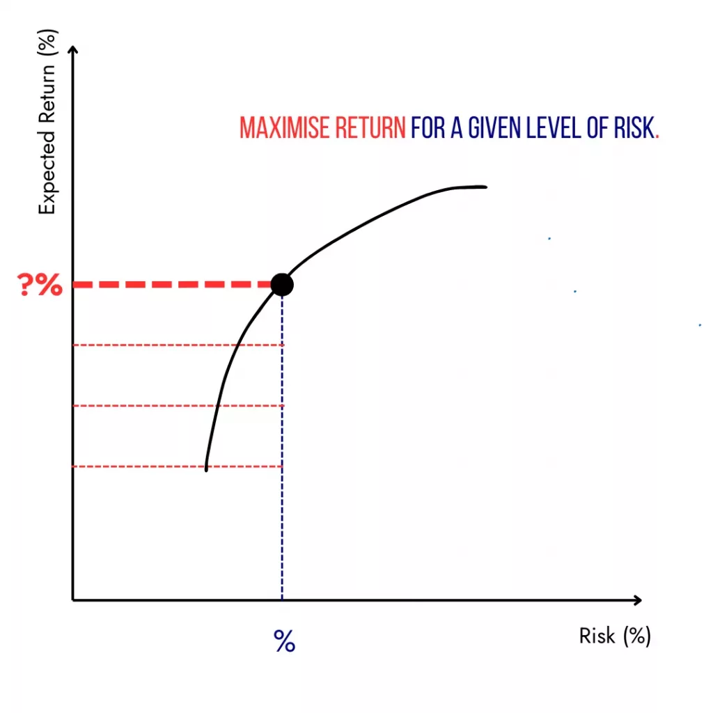

(A) (B)
Figure 1 Visualising the target problem in MVO: maximising return for a given level of risk (A), or minimising risk for a given level of return (B).
In practice, MVO method A is most popular because portfolio return has a simpler, linear formula (as the weighted average of individual returns) and therefore calculating the applicable weights when a risk value is already given is a much easier mathematical problem to solve. Method B on the other side requires the user to set the desired portfolio return and run much more complex portfolio risk calculations to determine the required weights.
What happens therefore in practice is that the investor (or the MVO tool) selects a range of portfolio risk values heuristically and calculates the weights that give the maximum expected return for each of the risk values, thereby creating the Efficient Frontier.
Maximising the Sharpe Ratio ((Expected return – Risk free rate of return) / volatility) gets a similar treatment, where volatility values are set, Risk free rate is a constant and the value “Expected return – Risk free rate of return” needs to be maximised for each risk value.
2.1. Lack of context gives uncertain answers
The major drawback to the MVO approach is that investors lack context, causing them to introduce their own bias/es when selecting the target return or target risk. They simply do not know if the target or the range of targets selected is the most accurate it could be.
MVO produces a curve (the Efficient Frontier, EF) and, depending on the specific tool implementation it may also give some context about where the current portfolio lies relative to the Efficient Frontier. See the example below.
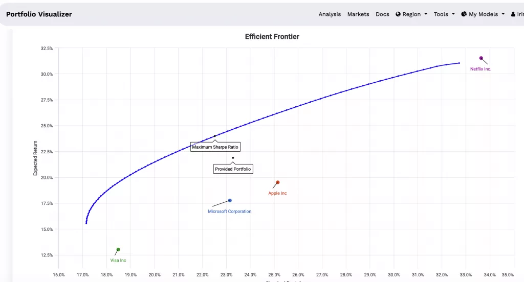
Figure 2 Visualising the Efficient Frontier in MVO when Maximum Sharpe Ratio optimisation was run
Figure 2 shows the Efficient Frontier created by a popular optimisation tool [6] where 100 points forming the frontier are plotted. The risk range was selected heuristically by the tool, and the point with the highest Sharpe value ratio is also highlighted.
With this approach the user does not know what other risk–return combinations are mathematically possible given the holdings universe and constraints.
Moreover, if the tool would make a less accurate selection of risk points (due to, for example, length or frequency of historical data points available for risk and correlation calculations), then the entire Efficient Frontier plot would be inaccurately placed on the two-dimensional risk return space.
Therefore, the user cannot be sure whether the point that was highlighted on an MVO derived frontier (e.g. the “maximum Sharpe ratio” in Figure 2) is a true, global maximum Sharpe for the portfolio OR it is only a local maximum Sharpe for the subset of 100 risk points selected by the tool.
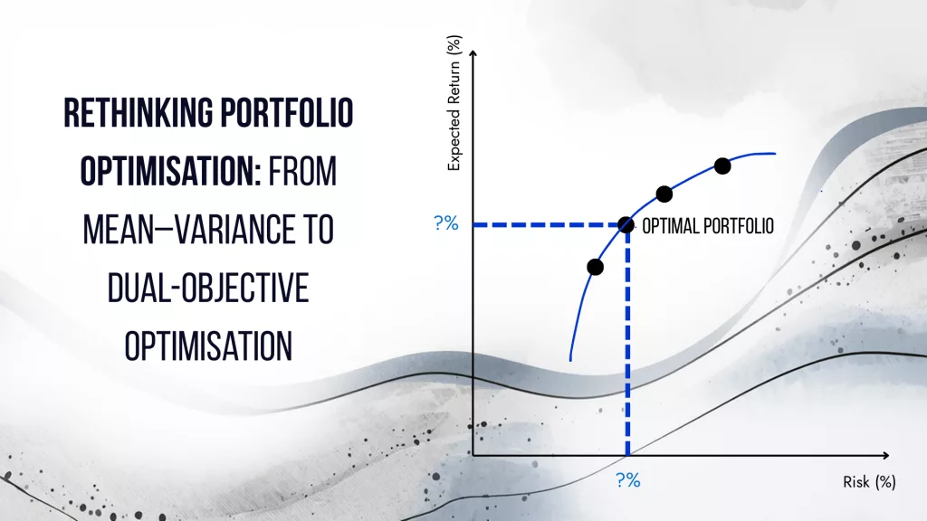
3. What DOOA Proposes: Simultaneous Optimisation and Solving for Risk and Return
3.1. Reframing the Objective
The Dual-Objective Optimisation Approach (DOOA) reframes the optimisation problem as a true bi-objective model: simultaneously minimise risk and maximise return. Instead of producing a frontier of efficient portfolios from which an investor must arbitrarily select one point, DOOA mathematically identifies a globally unique Efficient Frontier where the points on the frontier best balance the two objectives (risk and return) under the given inputs and constraints.
This formulation aligns with the intuitive goal of investment committees: find the most efficient set of weights that represents the best achievable combination of return and risk, not a menu of options requiring subjective choice.
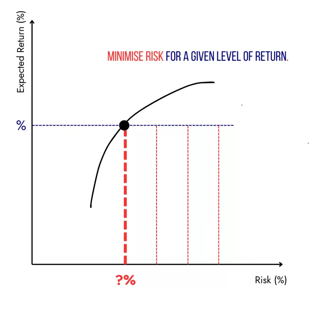
Figure 3 Visualising the target problem in DOOA: finding the allocation that maximises return and minimises risk at the same time
3.2. Visualising the Entire Universe of Possibilities
An essential feature of DOOA is its visual risk–return Portfolio Universe, which places the current portfolio within the full set of achievable positions (see example in Figure 4):
- A point representing the current allocation (with its risk and expected return),
- A scatter plot of a subset (up to 10K points) of all mathematically possible allocations given the asset universe and constraints,
- The Efficient Frontier as the top boundary of that universe,
- The Optimal Position as a point on the Efficient Frontier, along with the Minimum Risk Portfolio (also on the frontier, the leftmost point with lowest risk).
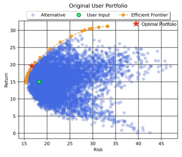
Figure 4 Example Portfolio Universe showing the current position (green point), other potential positions (blue points), Efficient Frontier positions (orange points) and the Optimal Portfolio (red star)
This visualisation delivers immediate clarity on what is possible, enabling more informed discussions about trade-offs than frontier curves alone.
Moreover, since DOOA considers the entire wide universe of risk-return positions for the portfolio, the user can be confident that the Optimal Portfolio or the Minimum Risk Portfolio, as required, is unique within that entire universe, for the constraints applied (if any).
3.3. Separation of Forecasting and Optimisation
DOOA also maintains a clear separation between:
- The Return forecasting – the expected returns used by the optimiser can be modelled using any preferred methodology (e.g., Black–Litterman, factor models, historical averages, proprietary research),
and
- The Optimisation engine – solving for the Optimal Position or other Efficient Frontier positions given the forecasted returns, volatility and correlations of the individual assets’ returns.
This modularity respects the governance and auditability requirements of professional asset management, where return assumptions should be transparent and distinct from optimisation mechanics.
3.4. Calculating expected returns using factor models
While it is not the purpose of this article to describe various types of method to calculate investments expected returns, a popular method deserves mentioning.
Calculating expected returns using factor models is a cornerstone of modern portfolio construction and a very popular approach used by practitioners. Rather than relying solely on historical averages, factor models decompose asset returns into underlying drivers, commonly referred to as “factors”, that explain systematic sources of risk and return.
The most widely known framework, the Capital Asset Pricing Model (CAPM), uses a single factor (the market risk premium) to estimate expected return. More advanced approaches, such as the the Fama-French-Carhart 5-Factor Model also consider various other factors to explain stock returns, aiming to better capture market anomalies. It includes company size, value growth, momentum, quality, and asset growth.
In these models, expected return is calculated as the sum of a risk-free rate plus the product of each factor’s expected premium and the asset’s sensitivity (beta) to that factor.
In practice, estimating expected returns with factor models involves both statistical analysis and forward-looking judgment. Historical data is used to estimate factor exposures and premiums, often via regression techniques, but practitioners must adjust these estimates to reflect current market conditions and expectations. This is particularly important because factor premiums are not constant over time and can vary across economic cycles.
For investment professionals, factor-based expected returns offer a more structured and transparent way to link portfolio construction to underlying economic drivers, enabling better-informed asset allocation, risk management, and performance attribution.
4. Example DOOA vs MVO
This sections shows how calculating the allocation for an efficient portfolio position using DOOA (Dual Objective Optimisation Approach) is more accurate than using MVO (Mean Variance Optimisation) and it is also able to increase the risk-adjusted return and Sharpe ratio for the portfolio.
For this example, the MVO tool used was PortfolioVisualizer [7], a popular software based in the US; for DOOA the tool used is Diversiview [8], a popular Australian software.
A summary of the example:
- First, the asset allocation that gives the maximum Sharpe Ratio is calculated using the MVO tool.
- Then, we analyse the portfolio created by the MVO tool in the DOOA tool , and show that the position identified by MVO is close but not on the Efficient Frontier, and
- Last, we calculate a more efficient Portfolio position on the Efficient Frontier using the DOOA tool, that gives a better Sharpe ratio.
Experiment settings and results
The selected multi-asset class portfolio consists of 11 ASX-listed ETFs, as follows: IOZ, IEM, HYGG, VGB, BILL, GLPR, CIIH, QRI, PE1, GOLD and VBND.
See the full list and the initial equal allocation in Figure 5 below.
The experiment was run on 12 April 2026; therefore, the data and indicators were valid at that time. Future runs of the same experiment might render different results as new daily pricing data and indicators become available.
To make sure that the results from the two tools are comparable (that is, any differences in the results could not be explained by different data inputs), both calculations using MVO and DOOA used the same expected returns and volatility values for the portfolio holdings.
Also, to allow fair comparison of the results, all optimised portfolio calculations were run with the same weighting constraints: min 5% and max 40% for any holding.
Step by step details:
A1) An optimisation is run in the MVO tool for the initial portfolio (equally weighted).

Figure 5 The initial portfolio with risk and expected return indicators, and the constraints applied
A2) The response from Portfolio Visualizer is retrieved. That is, the calculated portfolio position with maximum Sharpe ratio:
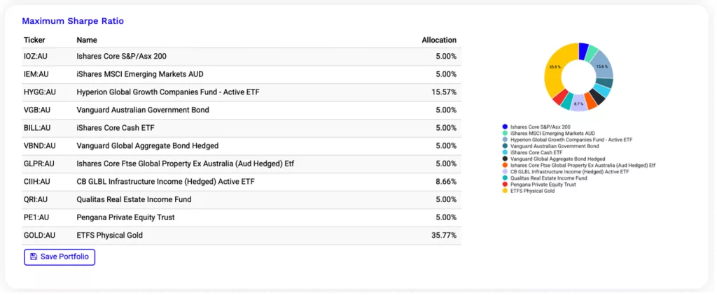
Figure 6 Calculated portfolio position with the highest Sharpe ratio, in the MVO tool
The MVO tool also produces a small Performance Summary table showing the indicators for the portfolio position.
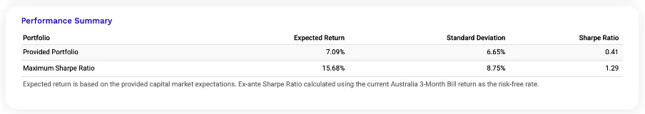
Figure 8 Portfolio indicators for the calculated portfolio position with maximum Sharpe ratio, in MVO
B1) The portfolio position produced by MVO tool is loaded into the DOOA tool.
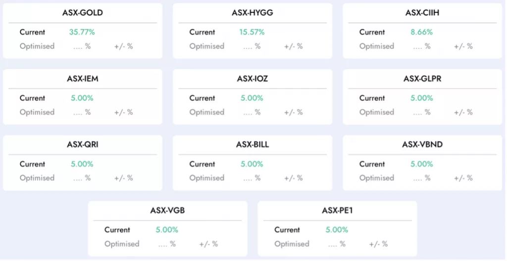
Figure 9 Max Sharpe portfolio position calculated by MVO is entered in DOOA tool
B2) Upon running the analysis of the MVO Max Sharpe portfolio in the DOOA tool, it can be noticed visually that in the Portfolio Universe produced by DOOA the portfolio position is not actually on the Efficient Frontier (see Figure 10, diagram on the right).

Figure 10 Portfolio indicators for the MVO-calculated position, in the DOOA tool
Sharpe ratio calculated by DOOA is 0.63, using the Australian Bond 10 years yield for the risk-free rate of return. Portfolio Beta is 0.34 and Portfolio Alpha is 0.05%.
Note, the portfolio volatility shows a big difference in DOOA compared with the MVO tool: from 8.75 % in the MVO tool to 24.92% in the DOOA tool. Portfolio Volatility is critical for the calculated Sharpe ratio.
One possible explanation could be that the MVO tool calculates correlations between pairs of investments using monthly returns for the shared history for all securities in the portfolio[1], whereas the DOOA tool calculates correlations based on daily returns for the past 10 years, where available, or full history where a security is younger than 10 years.
B3) A different, more efficient portfolio position is calculated using the “Efficient Frontier positions’ feature in the DOOA tool.
The result is analysed visually, and indicators compared, showing that the new position is more efficient (see Figures 11 and 12 below).

Figure 11 The new allocation for a more efficient portfolio position calculated by the DOOA tool

Figure 12 Portfolio indicators for a more efficient portfolio position calculated by the DOOA tool
While the Portfolio Expected return has reduced slightly by 0.49% (from 15.68% to 15.19%), all the other expected performance indicators show improvements:
- Portfolio Volatility has reduced from 24.92% to 23.60%
- Portfolio Sharpe ratio increased from 0.63 to 0.64
- Portfolio Beta has decreased from 0.34 to 0.31
- Portfolio Alpha has increased from 0.05% to 0.06%
While the increase in Sharpe ratio was not very large, it highlights two aspects:
a) more accurate calculations in DOOA tool compared with the MVO tool, and
b) the potential to increase the Sharpe ratio by finding position with significantly lower risk taken and a better Alpha.
5. Practical Implementation Considerations
Data Inputs
Like all optimisation frameworks, DOOA’s outputs are only as good as the inputs provided.
Practitioners should pay attention to a range of data aspects, particularly when comparing outputs from different optimisation tools, including but not limited to:
- the length of data considered,
- the frequency of data points (prices and/or returns),
- the type of instruments used for the risk free of return rates used in calculations
For example, using monthly vs daily historical returns will have a big impact on the calculated expected returns, volatility and correlations, which in turn will impact on the output allocation.
Similarly, using Australia 3-Month Bank Bill Swap Rate versus using Australia 10-year bond yield as the risk-free rate of return is likely to make a big difference for the indicators that use that rate.
Constraints and Business Rules
Real portfolios often incorporate cardinality constraints, minimum/maximum weight limits, and liquidity or regulatory limits. DOOA in Diversiview accommodates minimum/maximum weight limits transparently, with further types of constraints to be added soon. This makes it suitable for institutional mandates and model portfolio construction.
Integration into Workflow
Asset managers can embed DOOA into quarterly rebalancing workflows, model portfolio construction or risk reporting dashboards, offering auditable optimisation results.
6. Conclusion
Modern portfolio construction demands more than a curve. While Mean–Variance Optimisation remains foundational, its requirement for investors to pre-choose risk or return targets and its sensitivity to inputs can undermine decision quality.
The Dual-Objective Optimisation Approach (DOOA) advances beyond traditional MVO by treating risk and return as simultaneous goals, identifying a single optimal portfolio position that resides at the most efficient point in the attainable risk–return universe. It complements professional workflows by providing:
- Clarity of context through visual risk–return landscapes,
- Alignment with investor intuition (move up and/or left),
- Robust, stable allocations without arbitrary target setting,
- Flexibility in return forecasting inputs, and
- Governance-friendly separation of forecasting vs optimisation mechanics.
For asset managers seeking a more intuitive, robust, and professional optimisation framework, DOOA represents a pragmatic evolution of classical mean–variance methods, one that reflects both mathematical rigour and the practical realities of investment decision-making.
Readers who want to learn more about DOOA or the DOOA-enabled tool, Diversiview, can contact us at contact@lensellgroup.com with their questions or specific optimisation requirements.
References
- Markowitz, H. (1952). Portfolio Selection. The Journal of Finance, 7(1), 77–91. https://www.jstor.org/stable/2975974
- Diversiview (2026). Your Portfolio’s True Potential: Dual-Objective Optimisation Approach. https://diversiview.online/blog/your-portfolios-true-potential-dual-objective-optimisation-approach/
- Pappas, I., & Kontonikas, A. (2022). Mean-Variance Portfolio Optimisation: Challenges and Practical Considerations. MDPI Mathematics, 9(3), 223. https://www.mdpi.com/2227-7390/9/3/223
- Goltz, F., & Rieger, M. (2021). Multi-Objective Portfolio Optimisation Using CVaR and Other Risk Measures. MDPI Journal of Risk and Financial Management, 13(1), 15. https://www.mdpi.com/2227-7072/13/1/15
- Pflug, G. C., & Wozabal, D. (2007). Portfolio Optimization with Conditional Value-at-Risk: Theory and Practice. Journal of Banking & Finance, 31(6), 1627–1650. https://www.cambridge.org/core/services/aop-cambridge-core/content/view/9FBFDAB1B9FB4CF5E3E60EC9910A3731/S0973534810057172a.pdf
- Portfolio Visualizer, at PortfolioVisualizer.com
- Diversiview by LENSELL, at https://diversiview.online
- Fama, E. F., & French, K. R. (2015). A five-factor asset pricing model. Journal of Financial Economics, 116(1), 1-22.
[1] For example, if most securities in a portfolio are 5 years old and only one is 2 years old, the monthly returns for all securities for the past 2 years are used to calculate correlations in the exemplified MVO tool. Other MVO tools may give different results.
Disclaimer:
LENSELL GROUP Pty Ltd, ACN 646 467 941, trading as LENSELL, is a Corporate Authorised Representative of Foresight Analytics & Ratings Pty Ltd ( Australian Financial Services Licence No. 494552). All information provided to you by LENSELL is intended for general informational purposes only. It does not consider your individual financial circumstances and should not be relied upon without consulting a licensed investment professional or adviser.
The content on this website and in any of its applications is not a financial offer, recommendation, or advice to engage in any transaction. Investment products referenced in our software or marketing literature carry inherent risks, and you should note that past performance does not guarantee any future results. In all our modelling, no transaction costs or management fees are factored into performance analysis.
The information on our website or our mobile application is not intended to be an inducement, offer or solicitation to anyone in any jurisdiction in which LENSELL is not regulated or able to market its services.
Furthermore, all information used across our platform or website may be based on sources deemed reliable but is provided “as is” without guarantees of accuracy or updates. LENSELL and Foresight Analytics & Ratings disclaim all warranties and accepts no liability for any loss or damage resulting from use or reliance on any material or data embedded in our technology platform or digital media. Where liability cannot be excluded by law, it is limited to resupplying the information.
Please view our Financial Services Guide, Terms Of Service and Privacy Policy before making any investment decision using the information available on our website or on any of our applications. LENSELL, Diversiview and StockLenz are trademarks registered in Australia.